notebook: segmenting nuclei with the stardist napari plugin
Contents
notebook: segmenting nuclei with the stardist napari plugin#
Overview#
Plugins extend the functionality of napari and can be combined together to build workflows. Many plugins exist for common analysis tasks such as segmentation and filtering. In this activity, we will segment nuclei using the stardist napari plugin. Please visit the napari hub for a listing of the available plugins.
Data source#
The data were downloaded from the OpticalPooledScreens github repository.
Data source#
The data were downloaded from the OpticalPooledScreens github repository.
Loading the data#
We will start by loading an image of DAPI stained nuclei. We can use scikit-image’s imread() function to download the data from the link below and load it into a numpy array called nuclei.
from skimage import io

url = 'https://raw.githubusercontent.com/kevinyamauchi/napari-spot-detection-tutorial/main/data/nuclei_cropped.tif'
nuclei = io.imread(url)
Viewing the image#
As we did in the previous notebooks, we can view the image in napari using the napari.view_image() function. Here we set the colormap to magma.
import napari

viewer = napari.view_image(nuclei, colormap='magma')
from napari.utils import nbscreenshot

nbscreenshot(viewer)

Segment nuclei#
To segment the nuclei, we will use the stardist napari plugin. Please perform the segmentation using the instructions below. For more information on stardist, please see the papers and repository.
Start the stardist plugin. From the menu bar, click Plugins->stardist-napari:StarDist. You should see the plugin added to the right side of the viewer. Note it may take a while for the plugin to first open, as it downloads some pre-trained models for you.
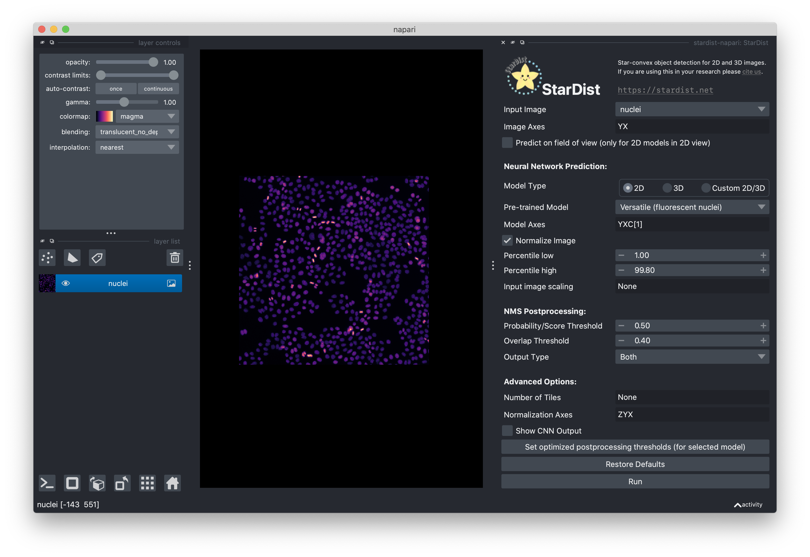
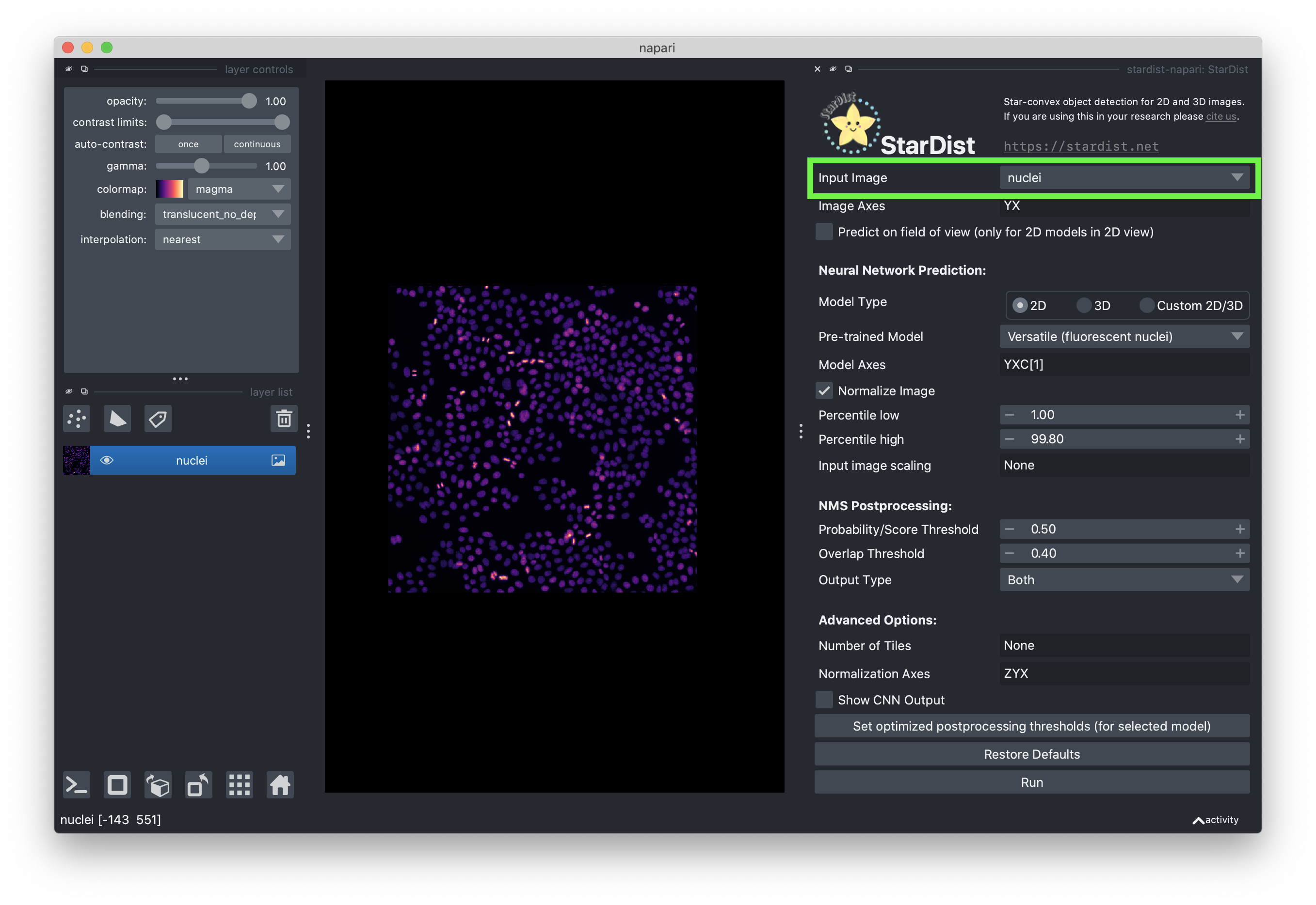
Select the “nuclei” image layer.
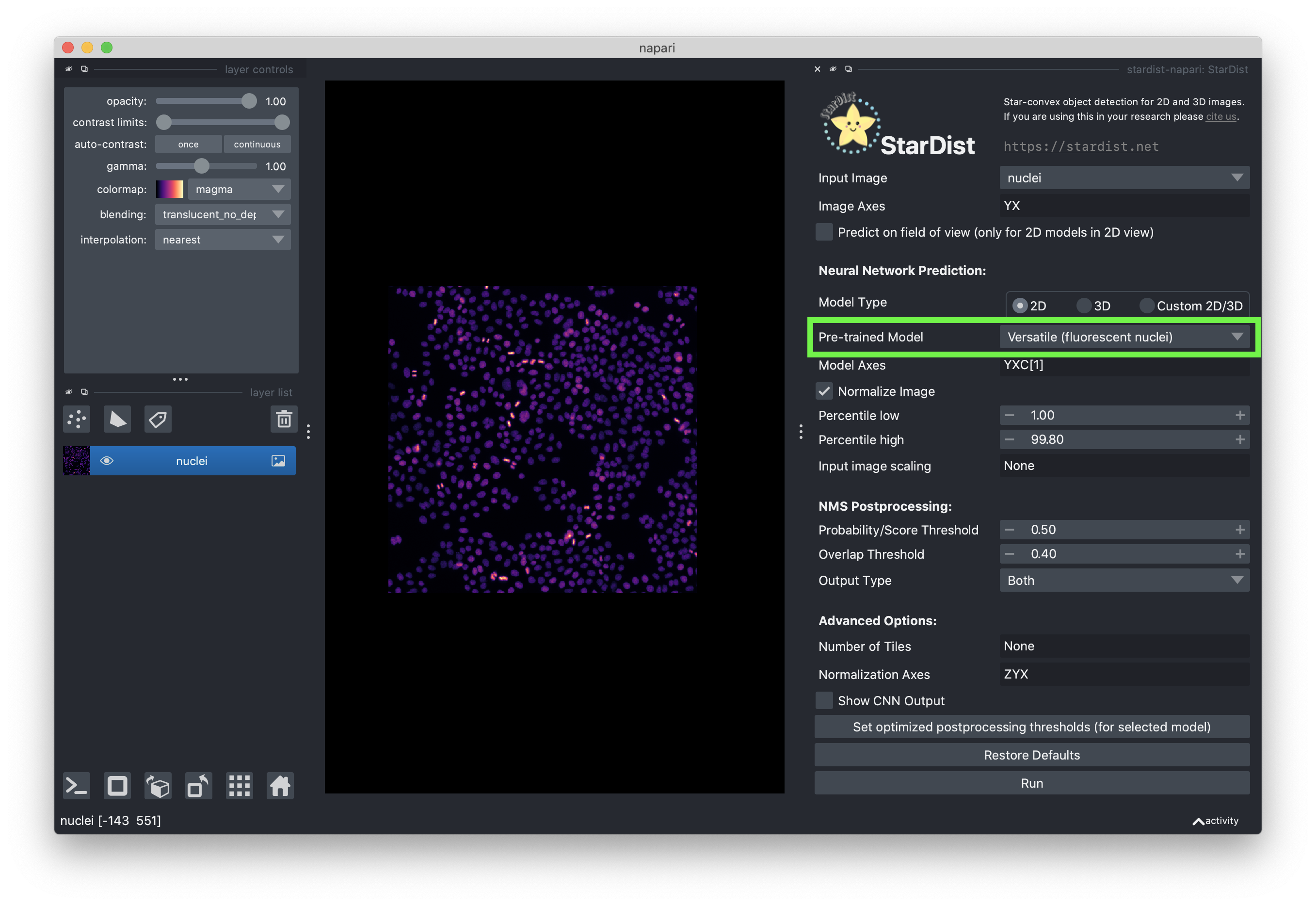
Set the model type to “2D”

Select the “Versatile (fluorescent nuclei)” pretrained model
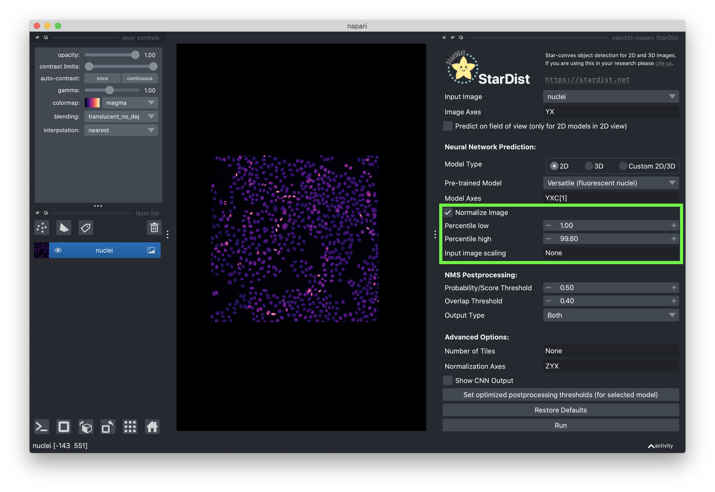
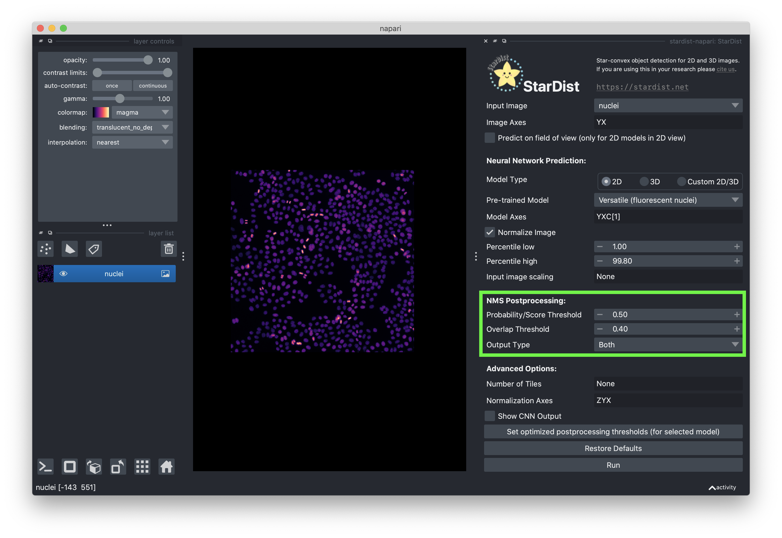
Check the “Normalize Image” checkbox and set the low and high percentiles to 1.00 and 99.80, respectively. Normalizing the image is important to ensure the intensity distribution is as similar as possible to the distribution the stardist model was trained on.
You can leave the postprocessing options as their default values. Setting the “Probability / Score Threshold” to higher values will likely reduce false positives, but also lead to fewer segmented objects. Increasing the “Overlap Threshold” will allow objects to overlap more. Feel free to play around with the settings!
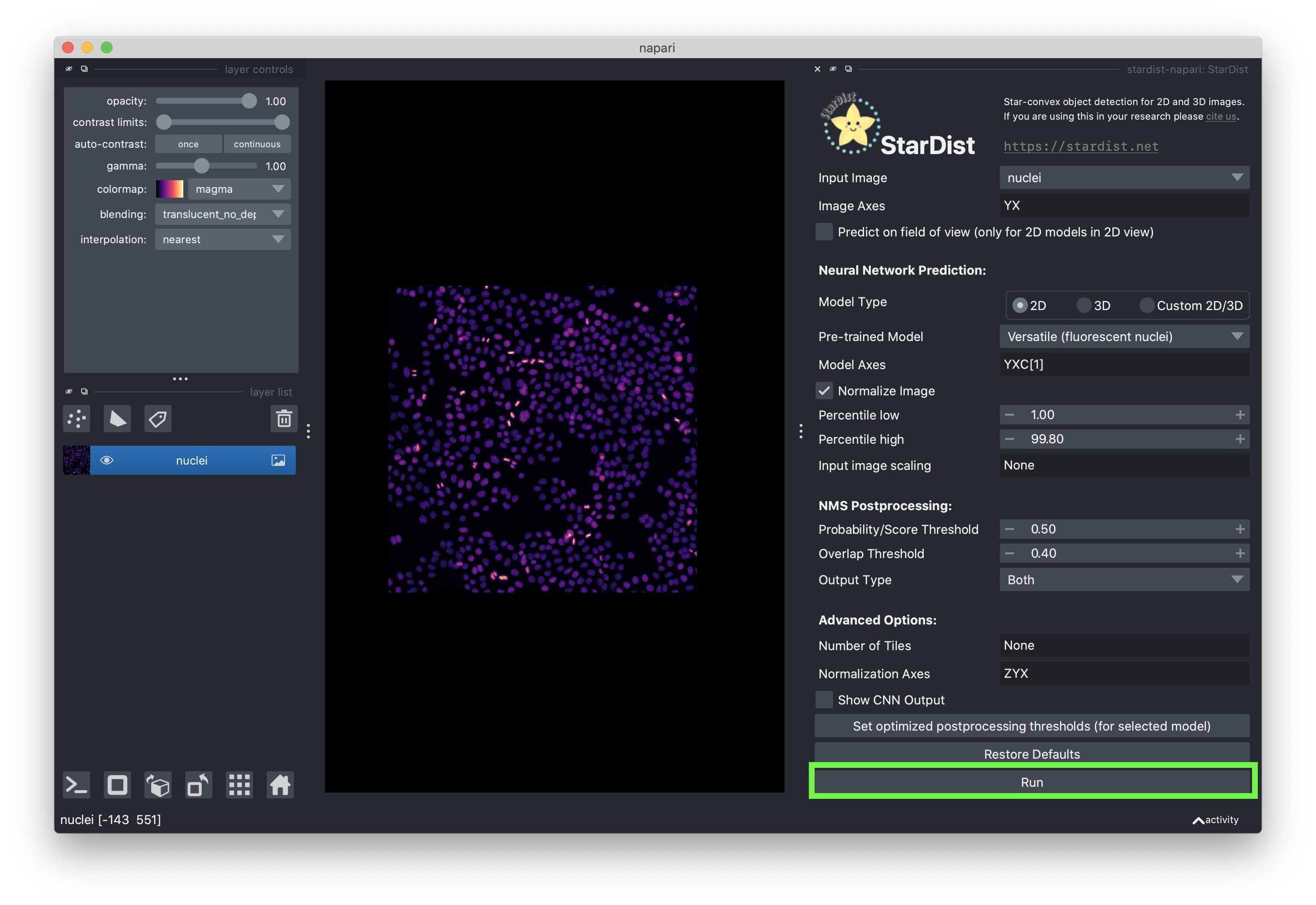
You can leave the “Advanced Options” as their default values
You are now ready to perform the segmentation! Press the “Run” button to start the segmentation. This may take a few minutes as we are running the computation on CPU. However, this would be much faster when using a GPU!
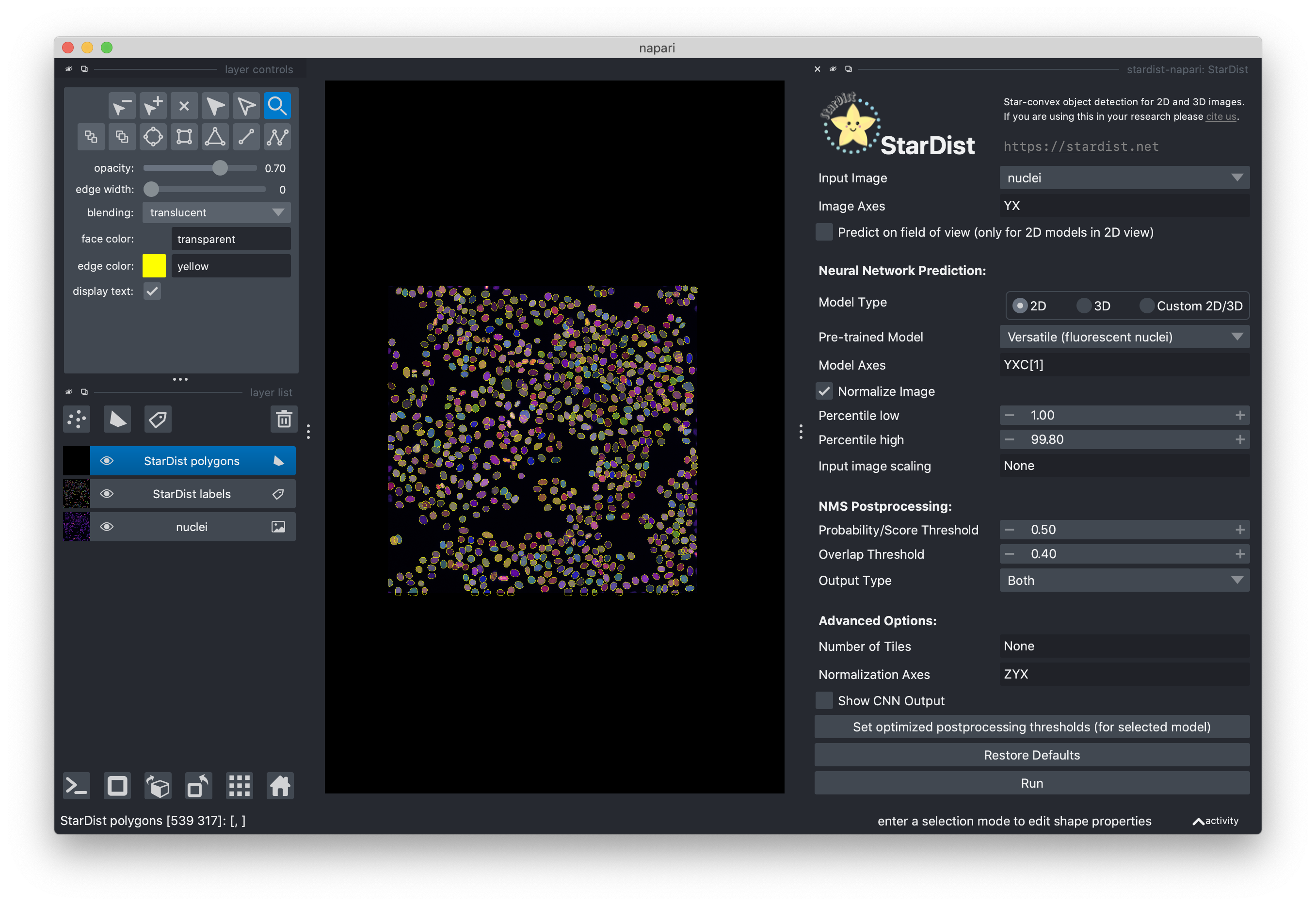
When the segmentation is complete, you should see the results in the viewer. Two layers have been added to the viewer. “StarDist polygons” contains the outlines of the segmented cells as polygons as a Shapes layer and “StarDist labels” contains the dense instance segmentation as a Labels layer.
Bonus: Quantify nuclei shape#
In this next section, we will compute and display some basic properties of the segmented cells (e.g., area) using scikit-image and matplotlib.
Measure area and perimeter#
stardist outputs the segmentation masks as a label image in a Labels layer called 'StarDist labels'. In napari, we can access the layer data from the layer object’s data property. As we did in the previous exercise, we can access the the layer object from the layer list by its name (viewer.layers['StarDist labels']). From that layer object, we can access the data.
We can use the scikit-image regionprops_table function to measure the area and perimeter of the detected nuclei. regionprops_table outputs a dictionary where each key is a name of a measurement (e.g., 'area') and the value is the measurement value for each detected object (nucleus in the case).`
from skimage.measure import regionprops_table

# measure the area and nucleus for each nucleus
label_layer = viewer.layers['StarDist labels']
rp_table = regionprops_table(
    label_layer.data,
    properties=('area', 'perimeter')
)
from matplotlib import pyplot as plt
import numpy as np
# print the median area
median_area = np.median(rp_table['area'])
print(f'median area: {median_area} px')
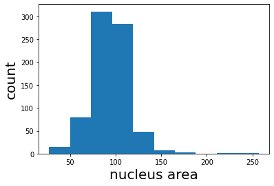
# plot a histogram of the areas
plt.hist(rp_table['area']);
plt.xlabel('nucleus area', fontsize=20);
plt.ylabel('count', fontsize=20);
plt.show();
median area: 94.0 px
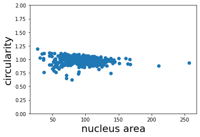
Finally, we can calculate the circularity from the area and perimeter measurements we made above. The circularity is a shape factor that is 1 when the object is a circle and less than one for shapes that are more “starfish-like”/ The circularity is defined as
where A is the area and P is the perimeter of the object. We plot the circularity vs. the area and see that the circularity of the nuclei does not appear to depend on the area.
# calculate the circularity of the nuclei
circularity = (4 * np.pi * rp_table['area']) / np.square(rp_table['perimeter'])

# use matplot lib to visualize the relationship between nucleus circularity and area
plt.scatter(rp_table['area'], circularity);
plt.xlabel('nucleus area', fontsize=20);
plt.ylabel('circularity', fontsize=20);
plt.ylim((0, 2))
plt.show()
Conclusions#
In this notebook, we have used the stardist-napari plugin to perform nucleus segmentation. We then used the results of the segmentation to inspect the relationship between nucleus area and circularity. This demonstration highlights how one can combine napari plugins and python libraries to make measurements on microscopy data.