notebook: bioimage visualization in python
Contents
notebook: bioimage visualization in python#
Python has a rich selection of data visualization tools that cover wide range of applications, for example Matplotlib (Hunter, 2007), Mayavi (Ramachandran & Varoquaux, 2011), ipyvolume, the yt Project (Turk et al., 2010), ITK (Johnson, McCormick, Ibanez 2015), and more recently napari.
For bioimage visualization some major challenges are:
working with large and complex images: image size and dimensionality
manual interactivity: for human in the loop annotation
interactive analysis: for interactive parameter tuning and quality control
This notebook will introduce napari a fast, interactive, multi-dimensional image viewer for Python.
Introducing napari#
napari is a fast, interactive, multi-dimensional image viewer for Python. It’s designed for browsing, annotating, and analyzing large multi-dimensional images. It’s built on top of Qt (for the GUI), vispy (for performant GPU-based rendering), and the scientific Python stack (numpy, scipy).
napari includes critical viewer features out-of-the-box, such as support for large multi-dimensional data, layering, and annotation. By integrating closely with the scientific Python ecosystem, napari can be easily coupled to leading machine learning and image analysis tools (e.g. scikit-image, scikit-learn, PyTorch), enabling more user-friendly automated analysis.
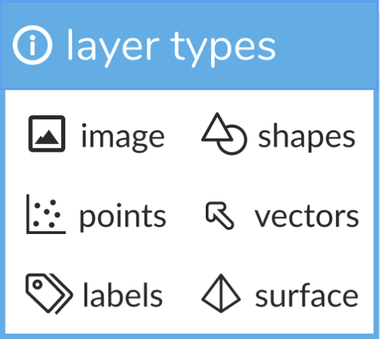
napari supports seven different layer types, Image, Labels, Points, Vectors, Shapes, Surface and Tracks. Each layer corresponds to a different data type and has it’s own set of visualizations and interactive controls. We provide an associated tutorial for each layer type to help you get started!
You can add multiple layers of different types into the viewer and work with them, adjusting their properties and performing analysis.
napari also supports bidirectional communication between the viewer and the Python kernel, which is especially useful when launching from jupyter notebooks or when using our built-in console. Using the console allows you to interactively load and save data from the viewer and control all the features of the viewer programmatically.
You can (and are encouraged to!) extend napari using custom key bindings, mouse functions, and our new plugin-interface.
Learn more about napari at napari.org, including our tutorials, our documentation and our mission and values.
Visualizing data with napari#
Let’s start by importing napari and creating an empty napari viewer
import napari
viewer = napari.Viewer()
Hopfully when you ran the above command a new empty napari viewer appeared in a seperate window.
Unlike other jupyter widgets, napari is not embedded inside the jupyter notebook. This is because the graphical parts of napari are written in Qt, making it hard to embed on the web.
Instead, we can take a screenshot of the current state of napari viewer and embed that in the notebook. This can be useful for teaching or sharing purposes where you might want to share key steps in an analysis which makes use of interactive components.
To do this, we use the nbscreenshot utility function
from napari.utils import nbscreenshot

nbscreenshot(viewer)

Note
Unfortunately, in contrast with the real napari viewer, these screenshots won’t be interactive!
Seeing our first image#
There are a few different ways to load images to into our viewer.
By
dragging and droppingimage files onto the viewerBy selection image files from the
Open File(s)menu optionUsing the
viewer.opencommand with a file path from within the notebookLoading the image data into an array and then passing that array using the
viewer.add_imagecommand
For the first three options the file path will get passed through our fileIO plugin interface, allowing you to easily leverage highly customized fileIO plugins for your diverse needs. The fourth option allows you complete control over loading and visualization and is most suited for when you have data already loaded into your notebook from other sources.
Here we will explore the fourth option, explicitly loading a 3D image using the scikit-image library and the add_image() method of our Viewer object.
from skimage.io import imread

# load the image data and inspect its shape
nuclei_url = 'https://raw.githubusercontent.com/alisterburt/napari-workshops/main/napari-workshops/notebooks/data/nuclei.tif'
nuclei = imread(nuclei_url)
print(nuclei.shape)
(60, 256, 256)
Now that we have the data array loaded, we can directly add it to the viewer.
## directly adding image data to the napari viewer
viewer.add_image(nuclei)
/Users/kyamauch/opt/miniconda3/envs/napari-tutorial/lib/python3.9/site-packages/napari/_vispy/vispy_camera.py:109: RuntimeWarning: divide by zero encountered in true_divide
  zoom = np.min(canvas_size / scale)
<Image layer 'nuclei' at 0x7fcac04e58b0>
Don’t forget to change windows so you can now see the viewer. By default you’ll just be looking at the 1st plane of the 3D data, which is the 0th slice of 60. You should see a single slider at the buttom of the viewer that will allow you to scroll through the rest of the z-stack. If you find the 30th slice then you should see the same as in the screenshot below.
nbscreenshot(viewer)

In the top left hand corner of the viewer we now have a control panel with controls that cover all our layers, and those that are specific to images like contrast limits and colormap.
Color channels and blending#
Right clicking on the contrast limits slider pulls up an elongated version of the slider which you can type specific numbers into. Let’s give that a try to adjust the contrast limits to [0.07, 0.35], and let’s change the colormap to blue using the drop down menu.
nbscreenshot(viewer)

One of the real strengths of napari is that you have full control over all the critical layer properties both programmatically and via the GUI.
Each layer that is added to the viewer can be found in the viewer.layers list.
# let's see what the layers list has in it right now
print(viewer.layers)
[<Image layer 'nuclei' at 0x7fcac04e58b0>]
The layer list can be indexed either numerically or by the layer name, which is visible in the panel in the bottom left of the viewer. This layer has the name nuclei, which was automatically imputed because we originally named the variable we loaded from disk nuclei. Pretty cool!
nuclei_layer = viewer.layers['nuclei']
first_layer = viewer.layers[0]
nuclei_layer, first_layer
(<Image layer 'nuclei' at 0x7fcac04e58b0>,
 <Image layer 'nuclei' at 0x7fcac04e58b0>)
If we go in and get the nuclei layer from our layer list we can now see and edit the values of some of the properties that we can control in the GUI.
# let's look at the values of some of the properties on the `nuclei` layer
print('Colormap: ', viewer.layers['nuclei'].colormap)
print('Contrast limits: ', viewer.layers['nuclei'].contrast_limits)
print('Opacity: ', viewer.layers['nuclei'].opacity)
Colormap:  colors=array([[0., 0., 0., 1.],
       [0., 0., 1., 1.]]) name='blue' interpolation='linear' controls=array([0., 1.])
Contrast limits:  [0.07, 0.35]
Opacity:  1.0
# Now let's change some of them. Note that the viewer GUI will update in real time as you run this code in the notebook
viewer.layers['nuclei'].colormap = 'red'
viewer.layers['nuclei'].contrast_limits = [0.4, 0.6]
viewer.layers['nuclei'].opacity = 0.9

# We can even rename the layer, but note that from now on you'll need to refer to if with its new name
viewer.layers['nuclei'].name = 'division'
nbscreenshot(viewer)

We could have actually passed these parameters as key-word arguments to during the first add_image call. For example we can add another copy of the data as follows:
viewer.add_image(nuclei, contrast_limits=[0.07, 0.35], colormap='blue', blending='additive')
<Image layer 'nuclei' at 0x7fcac0b11070>
Setting the blending of the second layer to additive now lets us see both together, which could be useful for understanding how parts of the image relate to each other.
nbscreenshot(viewer)

Let’s now load in an additional channel of data containing a stain for cell membranes and add them to the viewer as a new layer.
from skimage.io import imread

# load the image data and inspect its shape
membranes_url = 'https://raw.githubusercontent.com/alisterburt/napari-workshops/main/napari-workshops/notebooks/data/cell_membranes.tif'
membranes = imread(membranes_url)
print(membranes.shape)
(60, 256, 256)
viewer.add_image(membranes, contrast_limits=[0.02, 0.2], colormap='green', blending='additive');
nbscreenshot(viewer)

Orthogonal slicing and 3D rendering#
So far we’ve only looked at one slice. Use the slider at the bottom of the viewer to scroll through to another slice and see what the image looks like. For example the 45th slice looks like:
nbscreenshot(viewer)

As this is a 3D volume, we can also use napari to look at 2D slices along other axes. If we click the roll dimensions button in the bottom left hand corner of the viewer (which looks like a 3D cube with an arrow, 3rd from the left), and then scrolling through to the 60th slice gives the following:
nbscreenshot(viewer)

In addition to doing 2D rendering, napari can also do full 3D rendering. To enable 3D mode click on the 3D rendering button (which looks like a wireframe of a cube, second from the left). Now the slider has disappeared as the full 3D volume is being rendered at the same time. If the original dataset had been 4D, say for a volumteric timeseries then when using 2D rendering we would have initially seen two sliders, one for Z and one for Time, and 3D rendering would have switched us to only seeing one slider, for Time. In this way napari can be used to visualize either 2D or 3D slices of full n-Dimensional data with multiple color channels.
Try playing around with some of the 3D rendering modes and parameters in the gui to get a nice 3D visualization.
nbscreenshot(viewer)

Conclusions#
We’ve now seen how to use napari to visualize 3D images, including looking at 2D slices and the full 3D image. We’ve also learnt how to change properties of an image layer both from the GUI and from the jupyter notebook.
The next lessons will teach us how to create napari layers of other types, perform manual annotations, interactive analyses and more!